Improving Air Quality Comes with a Forecasting Twist

It’s been more than four years since we checked in with our partners at the NC Division of Air Quality about the state of air quality in North Carolina. Over the next two weeks, the NC DAQ team of air quality forecasters will offer some updates in a series of guest blog posts.
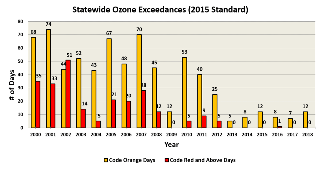
North Carolina’s air quality has improved dramatically over the past decade. This is especially true with regards to ozone concentrations. Prior to 2012, we typically saw 50 or more days each year in which our air quality monitors measured ozone concentrations above what the U.S. Environmental Protection Agency (EPA) has determined — through the latest scientific and medical research — to be unhealthy for sensitive groups (Code Orange on the Air Quality Index scale).
In 2012, there were 30 days where at least one monitor measured at or above the Code Orange range. That number has continued to decline annually since then, with each of the past 6 years having no more than 12 exceedance days when measured against the new, stricter 2015 ozone standard of 70 parts per billion. The decline in ozone is primarily due to the reduction in nitrogen oxide emissions from power plants and motor vehicles, which have fallen by more than 50% since 2002.
Success Gives Rise to a Challenge
The incredible reduction in ozone concentrations has been wonderful news for all North Carolinians, and everyone at the NC Division of Air Quality remains committed to working toward even better future air quality. However, for all of the benefits that our improved air quality has provided, it has also made our air quality forecasts increasingly complex and tough to communicate.
At first, it might seem counterintuitive to think that fewer poor air quality days can make air quality forecasting more difficult. The forecast ought to be easier now, right? Not so fast. The decrease in the frequency of days where ozone rises to unhealthy levels (Code Orange or worse) means that when those levels do occur, they tend to be more localized, and thus, harder to predict.
There are two main reasons why forecasting ozone at or above Code Orange levels has become so difficult. First, the nature of high ozone events is evolving. Historically, many of North Carolina’s worst air quality episodes (such as in June/July 2012) involved a large, significantly polluted air mass developing to our west or northwest before being slowly transported toward the state.
These large-scale high ozone events are akin to forecasting a hurricane or a winter storm once it’s evident on satellite and radar imagery. In other words, you can see it coming!
In recent years, due to improving air quality and how our summer weather patterns have taken shape, we have not seen many “transport events.” Instead, the few high ozone events in recent years have primarily been the result of local (in-state) emissions, and even the frequency of those events have been on the decline.
The second reason for more difficult high ozone forecasts has to do with what we have done within our own state to improve air quality. North Carolina has taken many steps to reduce the harmful emissions of nitrogen oxides that play a critical role in ozone formation.
As a result, when recent high ozone concentrations have occurred that were not due to a “transport event”, the corridors of higher ozone have been mostly confined to small, localized ozone plumes. These ozone plumes — small pockets of higher ozone concentrations — are primarily driven by local metropolitan emissions, and are now often on the order of only 10 to 20 miles wide!
These sorts of small-scale high ozone events are more comparable to trying to predict the precise location where a pop-up thunderstorm will form, or the exact location where a tornado will touch down. In other words, you cannot see it coming, and it forms in real-time with little to no advanced warning.
“Seeing” Ozone
Like any meteorologist, the way we “see” the phenomena we forecast is the same: our monitoring data. We rely heavily on air quality observations to help create forecasts for the coming days and to assess the accuracy of our forecasts later. If ozone levels are running higher or lower than expected on the current day, we can use that valuable information to supplement model forecasts and the vast amounts of meteorological data we process before making a forecast.
We have a network of more than three dozen ozone monitors across the state, with clusters of monitors located in and around the major metropolitan areas where ozone is most likely to form due to increased nitrogen oxide emissions.
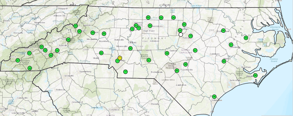
Our monitoring network at DAQ is designed and implemented to capture the trends in air quality over a period of years, as required by EPA regulations. It does a great job of showing how overall ozone concentrations are decreasing across the state and where we stand relative to the current ozone standard.
However, the increasingly localized nature of high ozone events means this network doesn’t always detect the highest concentrations within a forecast area, which is what our forecast predicts, especially if the wind isn’t blowing from the city or emission source toward a monitor. It’s a bit like casting a net into a lake. Even if we know that bass are in there, we may only catch minnows!
In our next post, we’ll provide a closer look at the process and data that goes into our daily air quality forecasts, including additional insights about the challenges of conveying this complex (but important!) information to the public.
In the third and final post of this series, we’ll have a Q&A about air quality topics including the 2018 ozone season, which featured a number of tricky forecasts and even trickier verifications. All in all, it was a great example of how our improving air quality has made life easier for just about everyone except air quality forecasters!
- Categories:


